#tidyTuesday, 1/18/2022, Chocolate

Exploratory Analysis

First, let’s examine the distribution of ratings of chocolates

milk_choc <- "#3d1c02"

ggplot(data = chocolate, mapping = aes(x = rating)) +
        geom_density(fill = milk_choc) +
        labs(title = "Distribution of Ratings") +
        theme_wsj() +
        theme(plot.title = element_text(size = 18))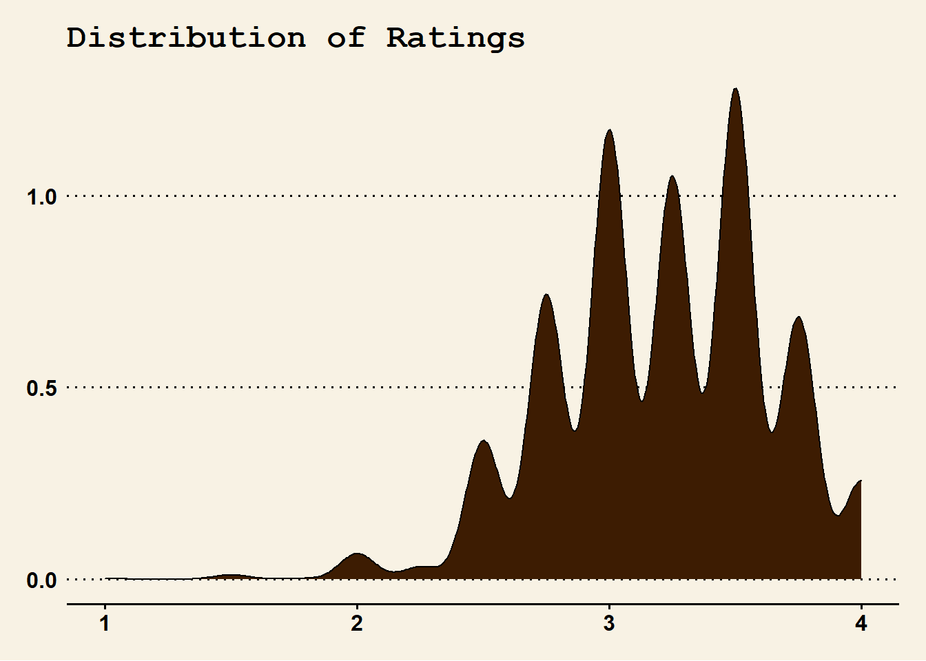

There are very few chocolates rated below a 2.2, which is interesting considering there are over 2500 observations.

Let’s explore the places where chocolate comes from.

country_count <- count(chocolate, country_of_bean_origin) %>%
        slice_max(n = 10, order_by = n)
ggplot(data = country_count, mapping = aes(x = reorder(country_of_bean_origin, -n), y = n)) +
        geom_col(color = milk_choc, fill = milk_choc) +
        theme_wsj() +
        labs(title = "Count of Country of Origin") +
        xlab("Country") +
        ylab("Count") +
        theme(axis.text.x = element_text(angle = -25, size = 10), plot.title = element_text(size = 18))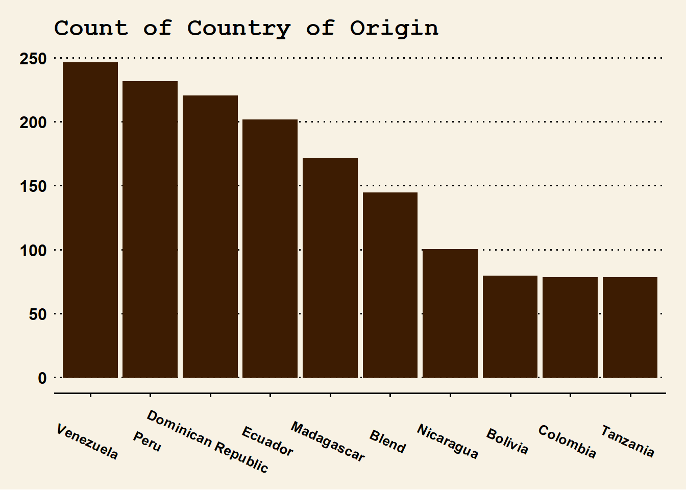

Central and South America are the dominant producers, with Madagascar and Tanzania thrown in.

That’s where the beans are produced. Where are the companies that produce the chocolate?

country_count <- count(chocolate, company_location) %>%
        slice_max(n = 10, order_by = n)
ggplot(data = country_count, mapping = aes(x = reorder(company_location, -n), y = n)) +
        geom_col(color = milk_choc, fill = milk_choc) +
        theme_wsj() +
        labs(title = "Count of Company Location") +
        xlab("Country") +
        ylab("Count") +
        theme(axis.text.x = element_text(angle = -25, size = 10), plot.title = element_text(size = 18))

The United States is by far the most productive. It’s interesting that Belgium and Switzerland are famous for their chocolate, but don’t really have very many or large companies.

Exploring Relationships

With that out of the way, let’s start exploring relationships. I’m primarily interested in the relationship between cocoa percent, ingredient count, and rating.

ggplot(data = chocolate, mapping = aes(x = cocoa_percent, y = rating, color = ing_count)) +
        geom_point() +
        geom_jitter(height = .5, width = .5) +
        theme_wsj() +
        labs(title = "Cocoa Percent vs. Ratings") +
        xlab("Cocoa Percent") +
        ylab("Rating") +
        theme(plot.title = element_text(size = 18), legend.title = element_text(size = 12)) +
        scale_color_gradient(name = "Ingredient Count", low = "#ead8bb", high = "#331100")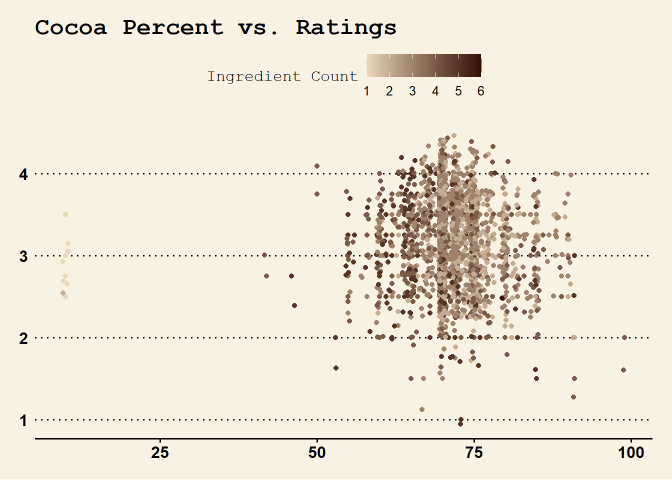

There doesn’t seem to be much of a relationship between these things. Let’s explore the relationship between country of bean origin and ratings.

top_avg_ratings <- chocolate %>%
        group_by(country_of_bean_origin) %>%
        summarize(avg_rating = mean(rating)) %>%
        slice_max(order_by = avg_rating, n = 10) %>%
        mutate(group = "Top Performers")

bot_avg_ratings <- chocolate %>%
        group_by(country_of_bean_origin) %>%
        summarize(avg_rating = mean(rating)) %>%
        slice_min(order_by = avg_rating, n = 10) %>%
        mutate(group = "Bottom Performers")

avg_ratings <- bind_rows(top_avg_ratings, bot_avg_ratings)

ggplot(data = avg_ratings, mapping = aes(x = reorder(country_of_bean_origin, -avg_rating), y = avg_rating, fill = group)) +
        geom_col() +
        theme_wsj() +
        labs(title = "Country of Origin vs. Mean Rating") +
        xlab("Country of Origin") +
        ylab("Mean Rating") +
        theme(plot.title = element_text(size = 18), legend.title = element_text(size = 12), axis.text.x = element_text(angle = -25, size = 10)) +
        scale_fill_manual(name = element_blank(), values = c("#6f5a48", "#662200"), guide = guide_legend(reverse = TRUE))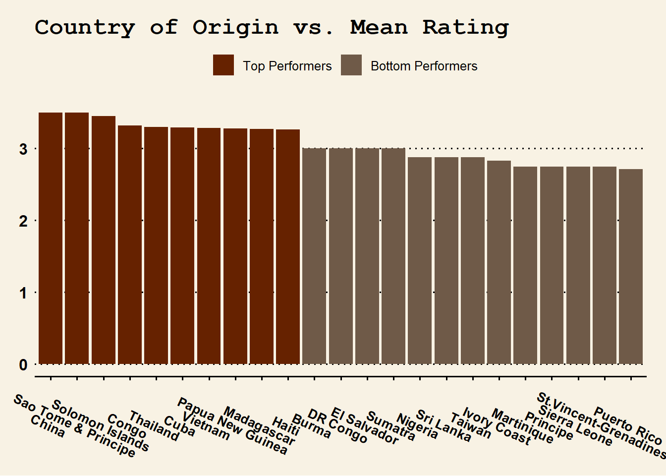

At first glance, it looks like only a few of our top 10 producers made it onto the top performer list. This is probably regression to the mean.

Language Processing

The most interesting feature to me is the “Most Memorable Characteristics”. Let’s look at the kind of words associated with chocolate

chocolate_words <- chocolate %>%
        select(most_memorable_characteristics) %>%
        unnest_tokens(characteristic, most_memorable_characteristics, token = 'regex', pattern = ',') %>%
        mutate(characteristic = str_trim(characteristic)) %>%
        count(characteristic) %>%
        slice_max(order_by = n, n = 25)


ggplot(data = chocolate_words, mapping = aes(label = characteristic, size = n, color = n)) +
        geom_text_wordcloud() +
        scale_size_area(max_size = 20) +
        scale_color_gradient(low = "#6f5a48", high = "#662200") +
        theme_wsj()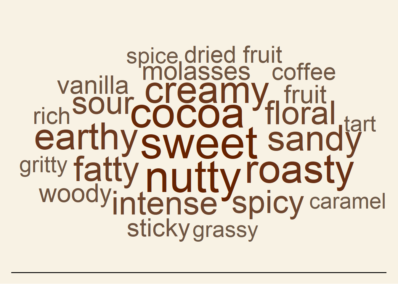

The most common words are sweet, cocoa, nutty, and roasty (I don’t know if that’s a word).

Finally, let’s explore the common words by rating.

words_with_ratings <- chocolate %>% 
        select(most_memorable_characteristics, rating) %>%
        group_by(rating) %>%
        unnest_tokens(characteristic, most_memorable_characteristics, token = 'regex', pattern = ',') %>%
        mutate(characteristic = str_trim(characteristic)) %>%
        count(characteristic) %>%
        slice_max(order_by = n, n = 5)
        

ggplot(data = words_with_ratings, mapping = aes(x = rating, y = n, label = characteristic, fill = n)) +
        geom_label() +
        theme_wsj() +
        theme(legend.position = 'none', plot.title = element_text(size = 21)) +
        labs(title = "Count of Characteristics by Rating") +
        xlab("Rating") +
        ylab("Count of Characteristic") +
        scale_fill_gradient(name = element_blank(), low = "#6f5a48", high = "#662200")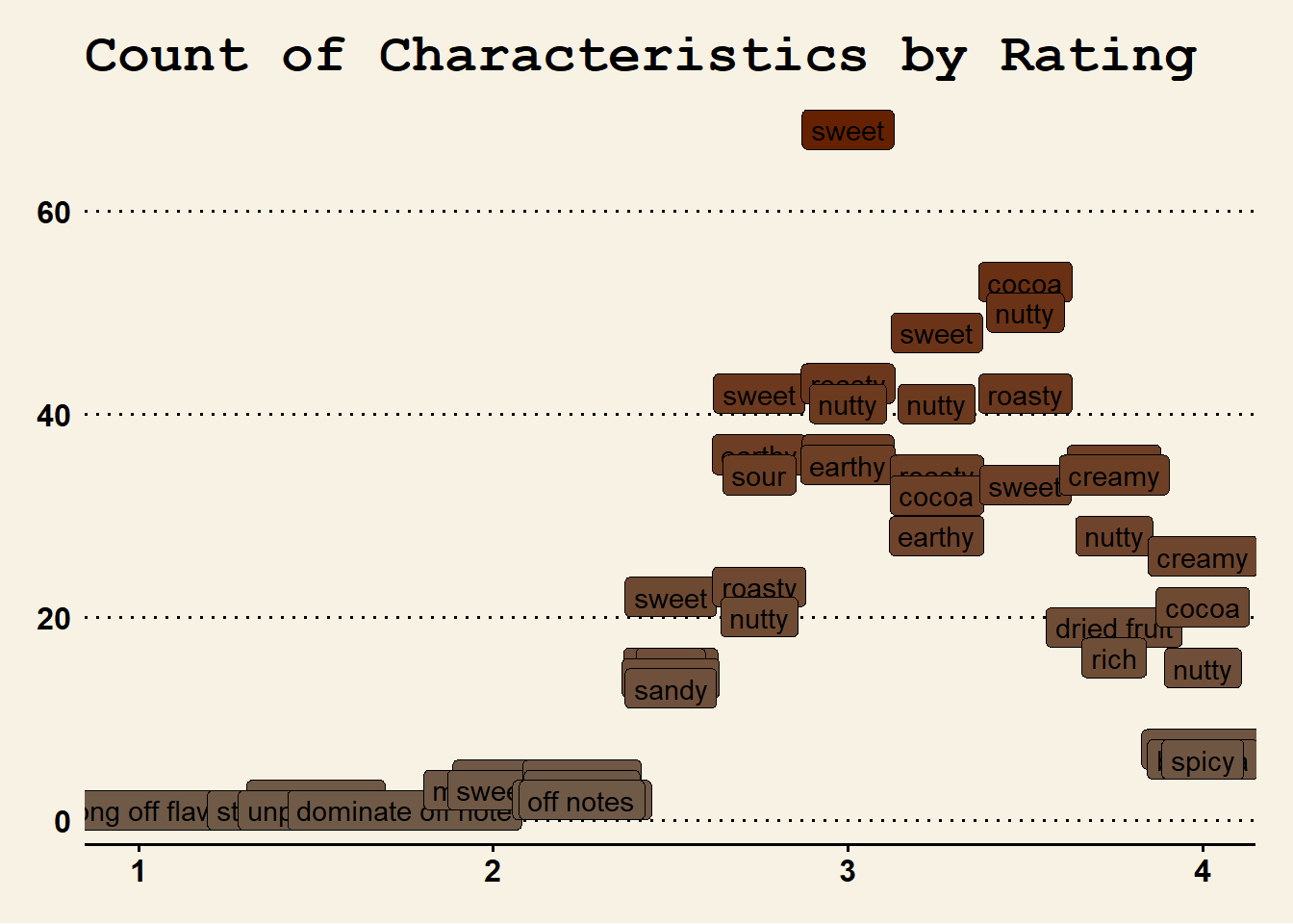

As ratings increase, it appears sweetness, nutty, creamy, and cocoa flavors are the most important.

Thanks for looking at my analysis!