#tidytuesday, 1/29/2022, Board Games

Exploratory Data Analysis

library(tidyverse)
library(tidymodels)
library(ggthemes)
library(ggrepel)
library(gganimate)

tuesdata <- tidytuesdayR::tt_load("2022-01-25")

## 
##  Downloading file 1 of 2: `details.csv`
##  Downloading file 2 of 2: `ratings.csv`

details <- tuesdata$details
ratings <- tuesdata$ratings


master <- inner_join(ratings, details, by = c("id" = "id")) %>%
        select(-c(num.y)) %>%
        rename(num = num.x)

First, let’s check the distribution of ratings across all games.

ggplot(data = master) +
        geom_density(mapping = aes(x = average), fill = "#014d64") +
        labs(title = "Distribution of Average Ratings") +
        xlab("Average Rating") +
        theme_economist()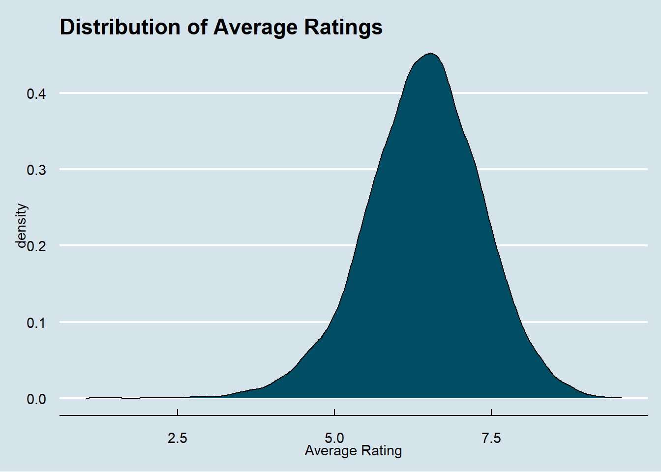

The average rating sits well above a 5 like we would expect. So either most games are better than average, or 5 isn’t the score a scorer would give an average game.

I’ve been playing around with animating plots recently to add some more interest to posts. Let’s explore how average ratings change by release year of the game.

There is an issue with the dataset where ancient games are causing some wackiness. I’m only going to include games made after 1950, with chess as a baseline to compare against.

ancient_games <- ratings %>%
        filter(!year %in% c(1950:2022),
               year != 2023)

modern_games <- ratings %>%
        anti_join(ancient_games) %>%
        group_by(year) %>%
        summarize(avg_rating = mean(average))

chess<- ratings %>%
        filter(id %in% c(171))

lowest_year <- modern_games %>%
        slice_min(order_by = avg_rating, n = 1)


year_plot <- ggplot(data = modern_games) +
        geom_line(aes(x = year, y = avg_rating)) +
        geom_point(aes(x = year, y = avg_rating))+
        #geom_point(data = lowest_year, aes(x = year, y = avg_rating), color = "#01a2d9") +
        #geom_label_repel(data = lowest_year, aes(x = year, y = avg_rating, label = year))
        geom_hline(data = chess, aes(yintercept = average, color = name)) +
        theme_economist() +
        labs(title = "Average Rating of Games vs Year", color = element_blank()) +
        ylab("Average Rating of All Games Released") +
        xlab("Release Year") +
        ylim(0,10) +
        scale_color_manual(values = c("#7c260b")) +
        theme(axis.title.x = element_text(vjust = -1), axis.title.y = element_text(vjust = 3)) + 
        gganimate::transition_reveal(modern_games$year)

animate(year_plot, renderer = gifski_renderer())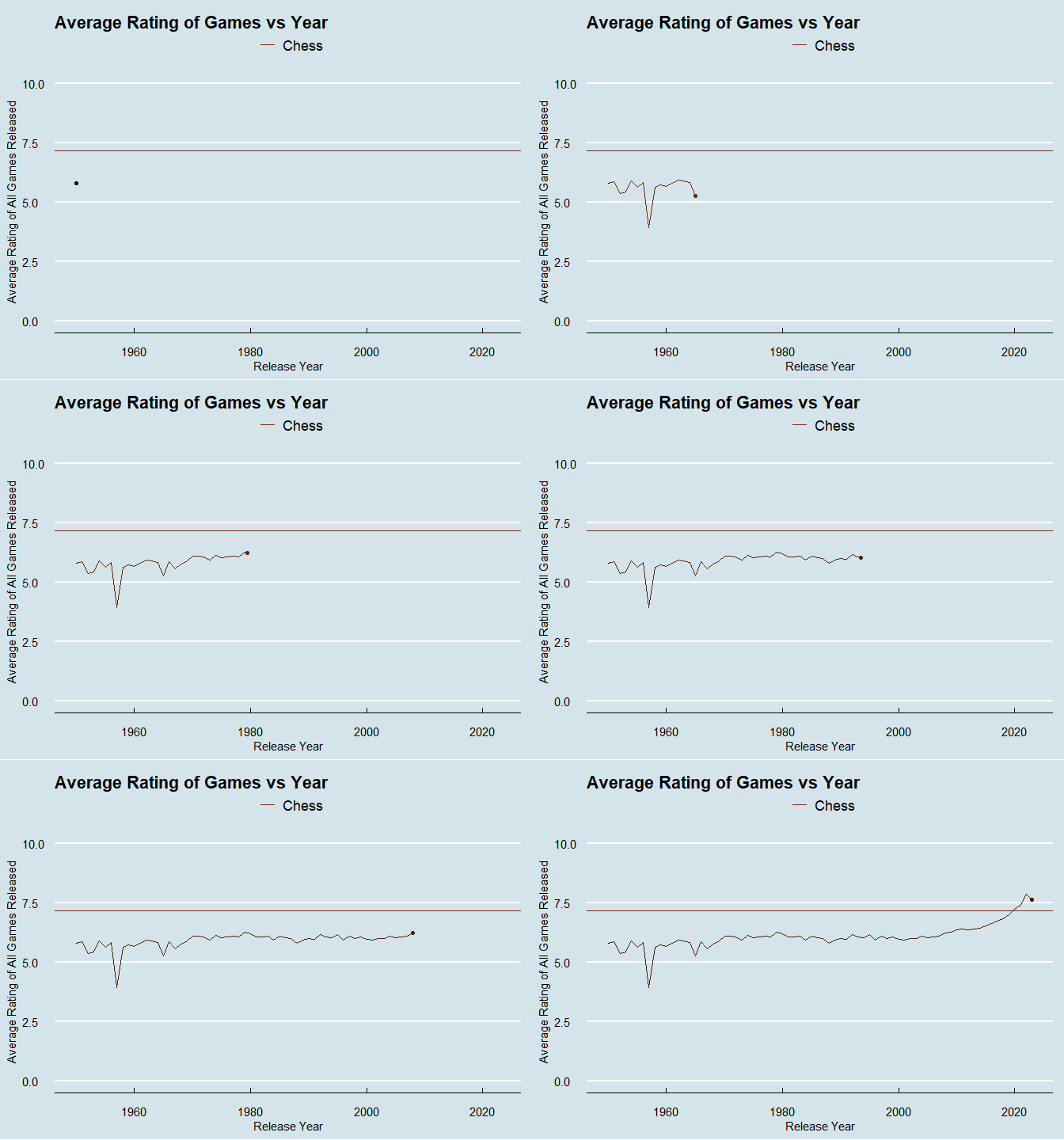

What was happening in 1957?

master %>%
        filter(year == 1957) %>%
        select(name, average, users_rated)

## # A tibble: 2 x 3
##   name                                average users_rated
##   <chr>                                 <dbl>       <dbl>
## 1 Don't Spill the Beans                  4.17         341
## 2 Curious George Match-a-Balloon Game    3.68          39

I probably wouldn’t rate these two games very high either.

Let’s look at ratings by game designer since 1980. This will be the top 10 most prolific designers.

designers <- master %>%
        mutate(designer = str_sub(boardgamedesigner, start = 3, end = -3)) %>%
        separate(designer, into = c("Designer"), sep = ",") %>%
        mutate(Designer = str_trim(str_replace_all(Designer, pattern = "'", "")),
               Designer = if_else(is.na(Designer), "(Uncredited)", Designer)) %>%
        filter(year %in% c(1980:2022)) %>%
        select(Designer, name, average)


designer_count <- designers %>%
        count(Designer, sort = TRUE) %>%
        slice_max(n, n = 10)

top_designers <- inner_join(designer_count, designers) %>%
        group_by(Designer) %>%
        summarize(mean_score = mean(average))



designer_plot <- ggplot(data = top_designers) +
        geom_col(aes(x = Designer, y = mean_score, fill = mean_score)) +
        theme_economist() +
        theme(axis.text.x = element_text(angle = -15, size = 8),
              axis.title.y = element_text(vjust = 2),
              legend.position = "None") +
        labs(title = "Average Score by Designer Since 1980") +
        xlab("Designer") +
        ylab("Average Score") +
        ylim(0,10) +
        transition_states(Designer, wrap = FALSE) +
        shadow_mark() +
        enter_grow()


animate(designer_plot, renderer = gifski_renderer())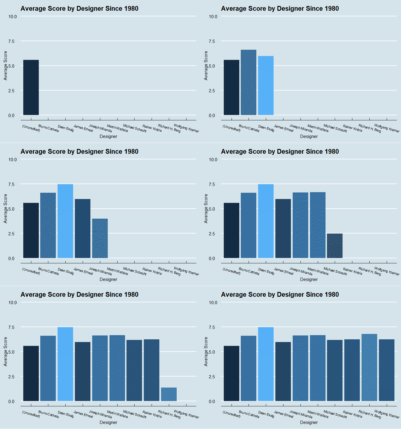

It’s interesting that most games go uncredited, and that these designers are so consistent with getting between a 6 and a 7.5 average score on their games

Model Building

Let’s build a model to predict the rating of the game based on the minimum number of players, maximum number of players, playtime, minimum play age, and the board game category.

I’ll be using an xgboost, and will be following Julia Silge’s tutorial for interpretability at https://juliasilge.com/blog/board-games/

Setting up the recipe:

set.seed(1337)

modified_master <- master %>%
        select(name, average, matches("min|max"), playingtime, boardgamecategory) %>%
        mutate(average = as.numeric(average)) %>%
        na.omit() %>%
        separate(boardgamecategory, into = c("prim_cat", "sec_cat", "ter_cat"), sep = ", ", ) %>%
        mutate(prim_cat = str_remove_all(prim_cat, "[:punct:]"),
               sec_cat = str_remove_all(sec_cat, "[:punct:]"),
               ter_cat = str_remove_all(ter_cat, "[:punct:]")) %>%
        replace(is.na(.), "None") %>%
        mutate_if(is.character, as.factor)

model_split <- modified_master %>%
        initial_split(strata = average)
        

board_training <- training(model_split)
board_testing <- testing(model_split)

straps <- vfold_cv(board_training, strata = average)
straps

## #  10-fold cross-validation using stratification 
## # A tibble: 10 x 2
##    splits               id    
##    <list>               <chr> 
##  1 <split [14407/1602]> Fold01
##  2 <split [14407/1602]> Fold02
##  3 <split [14407/1602]> Fold03
##  4 <split [14408/1601]> Fold04
##  5 <split [14408/1601]> Fold05
##  6 <split [14408/1601]> Fold06
##  7 <split [14408/1601]> Fold07
##  8 <split [14408/1601]> Fold08
##  9 <split [14410/1599]> Fold09
## 10 <split [14410/1599]> Fold10

boost_rec <- recipe(average ~ ., data = board_training) %>%
        update_role(name, new_role = 'ID') %>%
        step_other(all_nominal_predictors(), threshold = 5) %>%
        step_dummy(all_nominal_predictors(), one_hot = TRUE) %>%
        step_normalize(all_numeric_predictors())

prep(boost_rec)

## Recipe
## 
## Inputs:
## 
##       role #variables
##         ID          1
##    outcome          1
##  predictor          9
## 
## Training data contained 16009 data points and no missing data.
## 
## Operations:
## 
## Collapsing factor levels for prim_cat, sec_cat, ter_cat [trained]
## Dummy variables from prim_cat, sec_cat, ter_cat [trained]
## Centering and scaling for minplayers, maxplayers, minplaytime, maxplaytim... [trained]

and the model specifications:

boost_spec <- boost_tree(
        mtry = tune(),
        trees = tune(),
        min_n = tune(),
        loss_reduction = tune(),
        learn_rate = tune()
        ) %>%
        set_engine("xgboost") %>%
        set_mode("regression")

boost_spec

## Boosted Tree Model Specification (regression)
## 
## Main Arguments:
##   mtry = tune()
##   trees = tune()
##   min_n = tune()
##   learn_rate = tune()
##   loss_reduction = tune()
## 
## Computational engine: xgboost

and combining them to a workflow:

boost_flow <- workflow() %>%
        add_model(boost_spec) %>%
        add_recipe(boost_rec)

boost_flow

## == Workflow ====================================================================
## Preprocessor: Recipe
## Model: boost_tree()
## 
## -- Preprocessor ----------------------------------------------------------------
## 3 Recipe Steps
## 
## * step_other()
## * step_dummy()
## * step_normalize()
## 
## -- Model -----------------------------------------------------------------------
## Boosted Tree Model Specification (regression)
## 
## Main Arguments:
##   mtry = tune()
##   trees = tune()
##   min_n = tune()
##   learn_rate = tune()
##   loss_reduction = tune()
## 
## Computational engine: xgboost

library(finetune)

race <- tune_race_anova(
        boost_flow, 
        straps,
        grid = 15,
        metrics = metric_set(rmse),
        control = control_race(verbose = TRUE))

plot_race(race)

final_flow <- 
        boost_flow %>%
        finalize_workflow(select_best(race, 'rmse')) %>%
        last_fit(model_split)

collect_metrics(final_flow)

## # A tibble: 2 x 4
##   .metric .estimator .estimate .config             
##   <chr>   <chr>          <dbl> <chr>               
## 1 rmse    standard       0.730 Preprocessor1_Model1
## 2 rsq     standard       0.382 Preprocessor1_Model1

Let’s examine variable importance and how to interpret the variable importance.

library(vip)

boost_fit <- extract_fit_parsnip(final_flow)

vip(boost_fit, geom = "point") +
        theme_economist()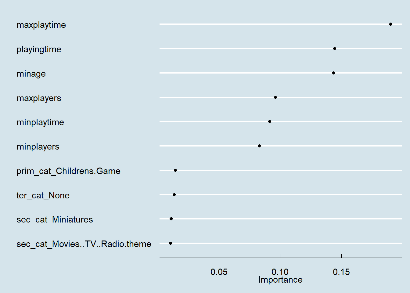

As far as xgboost goes, this is probably as descriptive you need to explain the model to stakeholders. If your stakeholders need additional explanation, a less “black box” model like a descision tree or multinomial logisitic regression is probably a safer bet.