#tidytuesday, 2/1/2022, Dog Breeds
First, dog tax:

Papi and Nana
Since last week we discussed interpreting a “black box” model like an XGBoost, I thought we could talk more about interpretability this week as well. Models have varying levels of interpretability and in some sense, all models are a black box to someone. To data scientists who (hopefully) know what’s going on behind the curtain, things aren’t so scary, but often stakeholders need to know how to act on the information that is gleaned from ML.
All models exist on a spectrum of interpretability, and generally interpretability and accuracy are negatively correlated. Neural networks, with the right setup, can be astonishingly accurate. There’s videos all over Youtube of no-hidden-layer networks solving what most people would consider to be complex problem spaces, like playing Asteroids. But watching the model work and explaining what it means when a certain node outputs a certain value are two different things.
I work in education. People want to know the relationships between things so they can act on it. If students are failing math at a particular school, they want a model to tell them why that may be the case, so they can make a plan to act on the information. Deploying a neural network would be an incredibly long uphill battle for me, since no one can “interpret” what each value at each node means at each layer.
Since we used a black box last week, I thought it would be nice to break out old-faithful:
Least Squares Linear Regression
EDA
library(tidyverse)
library(tidymodels)
library(ggthemes)
library(ggnewscale)
library(gganimate)
library(ggrepel)
library(shades)
library(ggcorrplot)

#tuesdata <- tidytuesdayR::tt_load("2022-02-01") This kicked back an error for some reason. I downloaded the data manually.
breeds <- read_csv("breeds.csv") %>%
janitor::clean_names() %>%
select(-c(links, image))
breeds_long <- breeds %>%
pivot_longer(cols = !breed, names_to = "year", values_to = "rank") %>%
mutate(year = as.numeric(str_sub(year, start = 2, end = 5)))
breeds_movement <- breeds %>%
drop_na() %>%
mutate(movement = x2020_rank - x2013_rank)
breeds_low_move <- breeds_movement %>%
slice_max(order_by = movement, n = 5) %>%
select(breed) %>%
inner_join(breeds_long)
breeds_high_move <- breeds_movement %>%
filter(sign(movement) == -1) %>%
slice_min(order_by = movement, n = 5) %>%
select(breed) %>%
inner_join(breeds_long)ratings_over_time <- ggplot(data = breeds_long, mapping = aes(x = year, y = rank, group = breed)) +
geom_point(alpha = .05) +
geom_line(alpha = .05) +
geom_point(data = breeds_low_move, mapping = aes(color = breed)) +
geom_line(data = breeds_low_move, mapping = aes(color = breed)) +
lightness(scale_color_brewer("Largest Decreases", palette = "Blues", guide = guide_legend(order = 2)), scalefac(.55)) +
new_scale_color()+
geom_point(data = breeds_high_move, mapping = aes(color = breed)) +
geom_line(data = breeds_high_move, mapping = aes(color = breed)) +
lightness(scale_color_brewer("Largest Increases", palette = "Reds", guide = guide_legend(order = 1)), scalefac(.55)) +
scale_y_reverse() +
labs(title = "Breed Rankings Over Time (2013-2020)") +
xlab("Year") +
ylab("Rank") +
transition_reveal(along = year)
animate(ratings_over_time, renderer = gifski_renderer(), end_pause = 20)
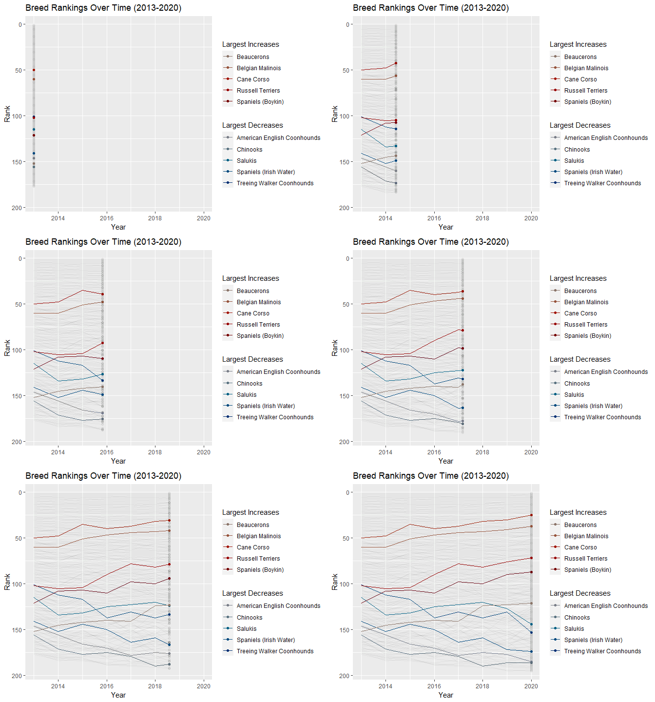
It is interesting how certain breeds moved such large spaces over the past few years. The Labrador retriever has been dominant as the AKC’s number 1 best dog. I don’t pay any mind to dog rankings or anything. Some breeds are naturally better at some things than others, but I adopt all my dogs, so I don’t worry about that sort of thing.
traits <- read_csv("traits.csv")

traits_long <- traits %>%
        select(-c('Coat Type', 'Coat Length')) %>%
        pivot_longer(cols = !Breed , names_to = "characteristic", values_to = "value")
ggplot(data = traits_long, mapping = aes(x = value, fill = characteristic)) +
geom_density()+
theme(legend.position = 'none') +
facet_wrap(~characteristic)
Very few of these are actually centered around 3 and leaning one way or the other. Only barking, coat grooming, and shedding level appear to be somewhat balanced. It looks like the others are perpetually good for all dogs.
Model Building
The goal is the most interpretable model possible. With that in mind, we aren’t going to preprocess our data at all, so that once the model is built we have a direct connection to the actual ranking.
traits <- read_csv("traits.csv") %>%
        janitor::clean_names() %>%
        select(-c(coat_type, coat_length))

ratings <- read_csv("breeds.csv") %>%
        janitor::clean_names() %>%
        select(breed, rank = x2020_rank)
cors <- round(cor(traits %>% select(-c(breed))), 1)
sig <- cor_pmat(traits %>% select(-c(breed)))
ggcorrplot(cors, outline.color = 'white', type = 'lower', p.mat = sig, color = c( "#313695", "white","#a50026"))
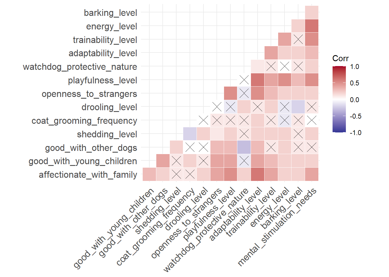
There are alot of correlated predictors though, so we will specify an interaction term between them.
master <- inner_join(ratings, traits)

dog_split <- master %>%
        initial_split(strata = rank)


dog_train <- training(dog_split)
dog_test <- testing(dog_split)

straps <- bootstraps(dog_train, strata = rank)
lm_rec <- recipe(rank ~ . , data = dog_train) %>%
update_role(breed, new_role = "ID") %>%
step_interact(all_numeric_predictors() ~ all_numeric_predictors())
prep(lm_rec)## Recipe
##
## Inputs:
##
## role #variables
## ID 1
## outcome 1
## predictor 14
##
## Training data contained 36 data points and no missing data.
##
## Operations:
##
## Interactions with affectionate_with_family + good_with_young_children + good_with_other_dogs + shedding_level + coat_grooming_frequency + drooling_level + openness_to_strangers + playfulness_level + watchdog_protective_nature + adaptability_level + trainability_level + energy_level + barking_level + mental_stimulation_needs affectionate_with_family + good_with_young_children + good_with_other_dogs + shedding_level + coat_grooming_frequency + drooling_level + openness_to_strangers + playfulness_level + watchdog_protective_nature + adaptability_level + trainability_level + energy_level + barking_level + mental_stimulation_needs [trained]lm_spec <- linear_reg() %>%
set_engine("lm") %>%
set_mode("regression")lm_flow <- workflow() %>%
add_recipe(lm_rec) %>%
add_model(lm_spec)fit <- fit_resamples(lm_flow, resamples = straps)
collect_metrics(fit)## # A tibble: 2 x 6
## .metric .estimator mean n std_err .config
## <chr> <chr> <dbl> <int> <dbl> <chr>
## 1 rmse standard 101. 25 8.84 Preprocessor1_Model1
## 2 rsq standard 0.0845 25 0.0151 Preprocessor1_Model1Is it a good model? No, it isn’t. In fact it’s practically worthless, but it is highly interpretable.
lm_final_flow <- lm_flow %>%
        finalize_workflow(select_best(fit, 'rmse')) %>%
        last_fit(dog_split)
lm_eng <- lm_final_flow %>%
extract_fit_engine()
lm_coeffs <- tidy((lm_eng$coefficients)) %>%
filter(names != "(Intercept)")ggplot(data = lm_coeffs, mapping = aes(x = names, y = x, label = names))+
ggrepel::geom_text_repel() +
geom_hline(aes(yintercept = 0), color = "midnightblue")+
theme(axis.text.x = element_blank(),
axis.title.x = element_blank(),
axis.ticks.x = element_blank()) +
labs(title = "Coefficients") +
ylab("Variable Coefficient")
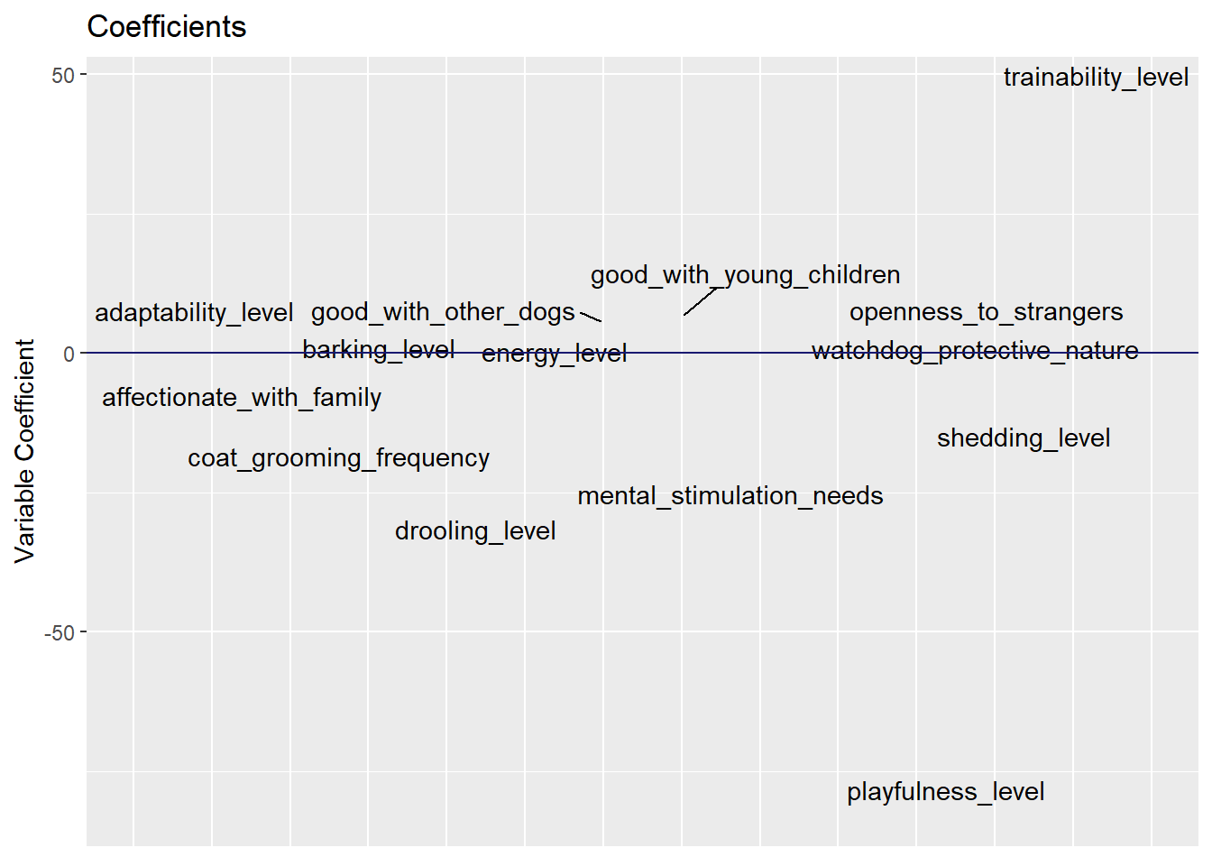
A dog being trainable, affectionate, good with children and open to strangers are all things that increase their ranking. A dog being too playful, drooling, and requiring too much mental stimulation are things that negatively impact the ranking, which all make sense.