Justice Analysis: San Fransisco Prosecutions

I’ve been out of the office a few days, and to start getting back into the groove of things I figured I would do an analysis of an interesting dataset. I found this data on Kaggle, and given my interest in criminal law, I thought it would make an interesting set.

library(tidyverse)

## -- Attaching packages --------------------------------------- tidyverse 1.3.1 --

## v ggplot2 3.3.5     v purrr   0.3.4
## v tibble  3.1.6     v dplyr   1.0.7
## v tidyr   1.2.0     v stringr 1.4.0
## v readr   2.1.2     v forcats 0.5.1

## Warning: package 'tibble' was built under R version 4.1.2

## Warning: package 'tidyr' was built under R version 4.1.2

## Warning: package 'readr' was built under R version 4.1.2

## Warning: package 'dplyr' was built under R version 4.1.2

## -- Conflicts ------------------------------------------ tidyverse_conflicts() --
## x dplyr::filter() masks stats::filter()
## x dplyr::lag()    masks stats::lag()

library(ggthemes)

cases <- read_csv('District_Attorney_Case_Resolutions.csv')

## Rows: 61515 Columns: 14

## -- Column specification --------------------------------------------------------
## Delimiter: ","
## chr  (9): incident_number, crime_type, filed_case_type, list_of_filed_charge...
## dbl  (2): court_number, disposition_code
## date (3): arrest_date, filing_date, disposition_date
## 
## i Use `spec()` to retrieve the full column specification for this data.
## i Specify the column types or set `show_col_types = FALSE` to quiet this message.

new_cases <- cases %>%
        janitor::clean_names() %>%
        filter(filing_date > as.Date("2011-12-31")) %>%
        select(arrest_date, filing_date, crime_type, filed_case_type, list_of_filed_charges, dv_case, disposition_date, case_status) %>%
        mutate(charge_count = str_count(list_of_filed_charges, ","),
               charge_count = charge_count + 1,
               arrest_to_file = filing_date - arrest_date,
               file_to_dispo = disposition_date - filing_date)

arrests_count <- new_cases %>% group_by(filed_case_type) %>%
        count(arrest_date, name = 'arrests') %>%
        rename(date = arrest_date)

file_count <- new_cases %>% group_by(filed_case_type) %>%
        count(filing_date, name = 'filings') %>%
        rename(date = filing_date)

dispo_count <- new_cases %>% group_by(filed_case_type) %>%
        count(disposition_date, name = 'dispos') %>%
        rename(date = disposition_date)


case_counts_by_date <- arrests_count %>%
        full_join(file_count) %>%
        full_join(dispo_count) %>%
        replace(., is.na(.), 0) %>%
        ungroup() %>%
        filter(date > as.Date("2011-12-31")) %>%
        pivot_longer(cols = c(arrests, filings, dispos), names_to = "type", values_to = "count") %>%
        mutate(type = case_when(
                type == 'arrests' ~ 'Arrests',
                type == 'filings' ~ 'Filings',
                type == 'dispos' ~ 'Dispositions'
        )) %>%
        mutate(type = as_factor(type))

## Joining, by = c("filed_case_type", "date")
## Joining, by = c("filed_case_type", "date")

case_counts_by_date$type = fct_relevel(case_counts_by_date$type, c('Arrests', 'Filings', 'Dispositions'))

colors = c("Felony" = "#ee8f71", "Misdemeanor" = "#014d64")

ggplot(data = case_counts_by_date) +
        geom_line(mapping = aes(x = date, y = count, color = filed_case_type), alpha = .7) +
        theme_economist() +
        scale_color_manual(values = colors, name = "Filed Case Type") +
        facet_wrap(vars(type), nrow = 3, ncol = 1, scales = 'free_y') +
        labs(title = "Counts of Action taken by SF Police/DA Over time") +
        xlab("Time") +
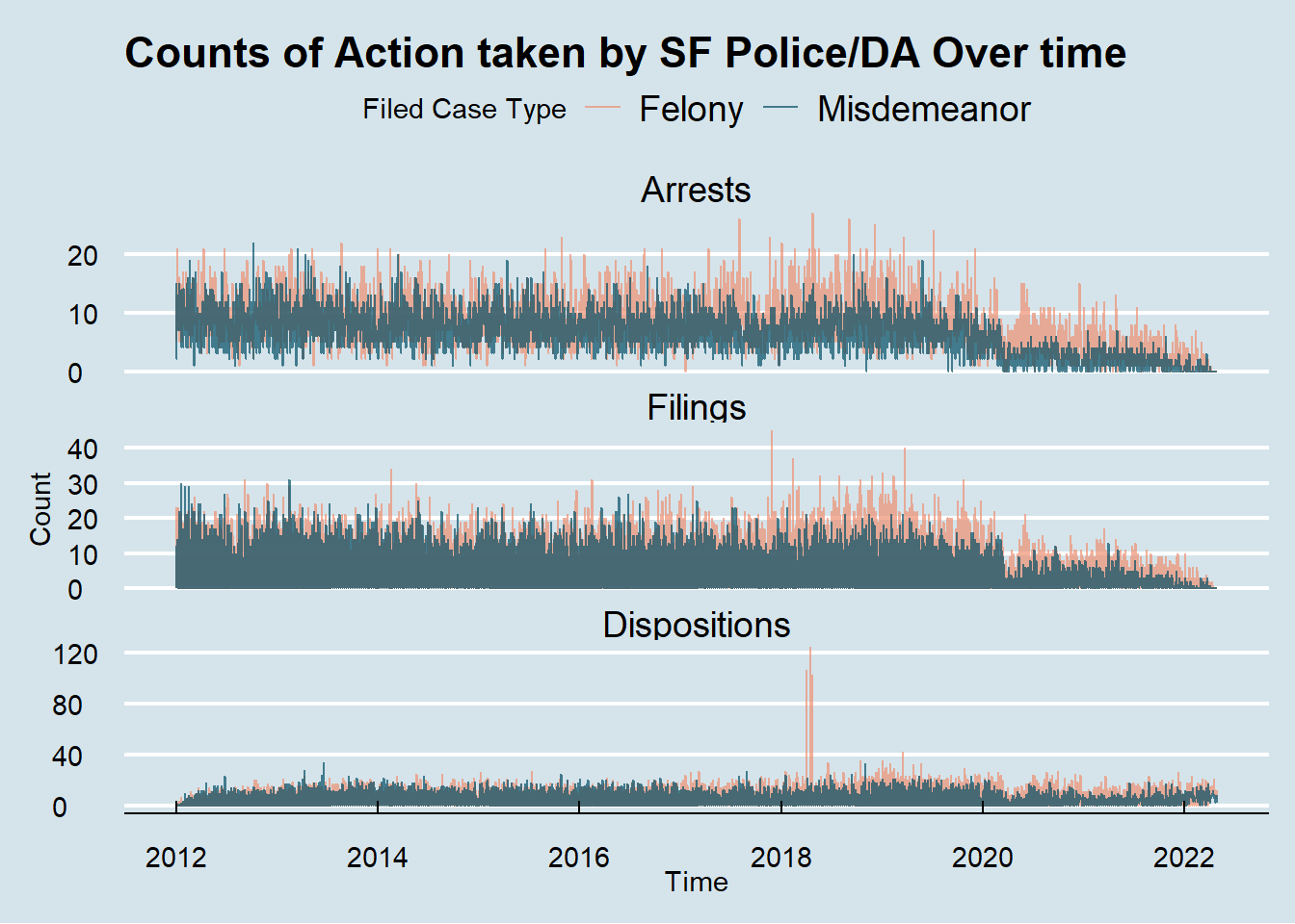
        ylab("Count") 

First, we can explore the count of actions taken by the Police and DA over time. We can see that there was a huge spike in dispositions during the beginning of 2018. There are also consistently more filings than arrests on any given day. We can also very clearly see the drop in everything at the start of the pandemic, and it’s interesting it hsan’t really recovered.

date_move <- new_cases %>%
        pivot_longer(cols = c(arrest_to_file, file_to_dispo), names_to = "type", values_to = "value") %>%
        select(arrest_date, filed_case_type, type, value) %>%
        mutate(type = case_when(
                type == "arrest_to_file" ~ "Arrest to File Date",
                type == "file_to_dispo" ~ "File to Dispo Date"
        ))

colors = c("Arrest to File Date" = "#ee8f71", "File to Dispo Date" = "#014d64")

ggplot(data = date_move) +
        geom_line(mapping = aes(x = arrest_date, y = value, color = type), alpha = .5) +
        theme_economist() +
        scale_color_manual(values = colors, name = "") +
        facet_wrap(vars(filed_case_type), nrow = 2, ncol = 1) +
        theme(axis.title.y = element_text(vjust = 4)) +
        labs(title = "Time Between Actions") +
        xlab("Time") +
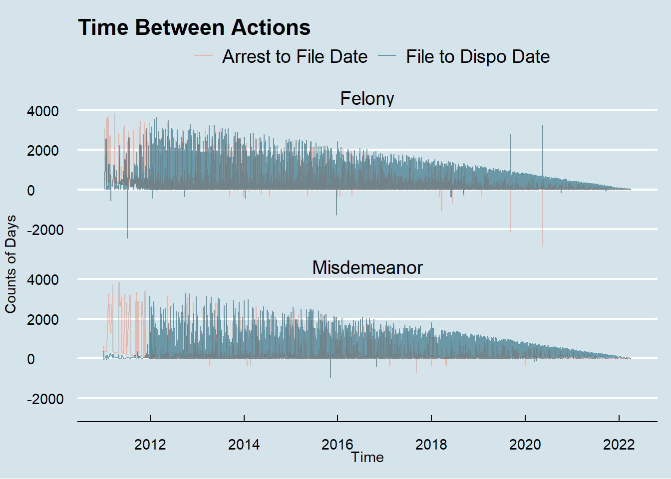
        ylab("Counts of Days")

## Don't know how to automatically pick scale for object of type difftime. Defaulting to continuous.

Next we can look at the time between actions taken. We can see often the time between filing and a disposition is much longer than the time between arrest and filing, and misdemeanors take less time than felonies, as we would expect to be the case. There are also rare occasions where there is a filing prior to arrest, which makes sense. There are some strange issues where there is a disposition before filing, which doesn’t make sense.